Parameter atlas — flip through all 15 maps in place
0.1° global fields (seed s1, the canonical release), 50 m coastlines, robust 2–98% stretch. Use ← → keys, the arrows, or click a parameter chip. Titles carry meaning, unit, box and global median.

1,178,590 land cells × 15 parameters, learned end-to-end from 7,855 GRDC+Caravan stations through differentiable CREST physics, forced purely by IMERG. Shipped as two fields (yardstick-optimal + physics-hardened) with a per-cell confidence layer. Every number below is a paired-Wilcoxon, multi-seed verdict.
▶ Report deck (in-page, 13 slides) 🗺 Parameter atlas (15 maps)
| Component | What it is | Evidence |
|---|---|---|
| Field A — yardstick-optimal | CNN head (two 3×3 conv, 256 ch) on 22 covariates; no physics constraint. For continents with training stations. | ungauged 0.514 (runs 0.503/0.514/0.519/0.514/0.529, plateau ≥480 iters) |
| Field B — extrapolation-hardened | Same + Budyko weak supervision (BUDW=100) applied to basins whose discharge never enters the loss. For data-sparse / regime-novel regions. | leave-continent-out: SA +0.09, AF +0.05 (paired, p<1e-5); yardstick price −0.02 (0.490±0.003) |
| Confidence layer | Per-cell [0,1]: 3-seed dispersion × covariate coverage × continent LRO prior | tells users which field to trust where |
| Routing tier | Gamma UH per basin <50k km²; differentiable Muskingum–Cunge above | big-basin tier (213 st.): ungauged 0.324; mid-tier test: UH wins below 50k |
| Head network rule | CNN in-distribution only; MLP head for continental extrapolation | CNN off-continent collapses (LRO-SA −0.49); MLP loses only 0.014 (EU) – 0.21 (OC) |
recipe CRESTPhys + tension store (ft) + learnable Gamma UH · Snow-17 defaults · robust KGE loss (tail-capped + β penalty) · 480 full-batch iterations · train 2012–23, evaluate 2003–11 · IMERG V07 daily, ERA5 lapse-corrected T, Oudin PET — every input exists globally with no gauges.
| Metric | IMERG (product) | MSWEP (diagnostic) |
|---|---|---|
| daily KGE | 0.514 | 0.605 |
| monthly KGE | 0.603 | 0.641 |
| daily NSE | 0.369 | 0.505 |
| β (bias) | 0.98 | 0.96 |
| ceiling (per-station calib.) | 0.579 | 0.650 |
MSWEP embeds rain-gauge information (+0.05 premium) that does not exist in truly ungauged regions — IMERG is the deployable line, MSWEP bounds what gauge-informed forcing would add.
| Slice | KGE |
|---|---|
| N. America / Europe | 0.565 / 0.529 |
| S. America / Africa / Oceania | 0.485 / 0.438 / 0.394 |
| area <500 → 10–50k km² | 0.464 → 0.599 |
| wet / mid / dry | 0.558 / 0.555 / 0.407 |
Africa 0.12 → 0.44 across versions is the largest jump. Asia ships as labeled extrapolation (MLP + hardened field) until CAMELS-IND ingestion.
| Param | Meaning | Unit | Mode | Box | Provenance |
|---|---|---|---|---|---|
| wm | Max soil water capacity (VIC b-curve mean) | mm | mult ×⅓–3 | 1–2000 | classic CREST |
| b | b-curve exponent (sub-cell heterogeneity) | – | mult ×⅓–3 | 0.01–6 | classic CREST |
| im | Impervious fraction | – | mult ×0.2–5 | 0–0.5 | classic CREST |
| fc | Infiltration capacity (fixed at prior) | mm/hr | fixed | 0–150 | classic CREST |
| ke | PET adjustment | – | direct | 0.2–2.5 | classic CREST |
| ksoil | Soil→aquifer drainage rate | 1/day | mult ×0.2–5 | 0–0.5 | CRESTPhys |
| hmaxaq | Aquifer capacity (fill-and-spill) | mm | mult ×⅓–3 | 50–4000 | CRESTPhys |
| gwc / gwe | Baseflow coefficient / exponent | mm/d · – | direct | 0.01–5 · 0.5–6 | CRESTPhys |
| ft ★ | Tension-store fraction of wm | – | mult ×⅓–3 | 0–0.7 | this work |
| qc | Surface linear-reservoir release | 1/day | direct | 0.05–1 | this work (operator-bound) |
| nshape / kmult | Gamma UH shape / time-scale multiplier | – | direct | 1–8 · 0.1–4 | this work (operator-bound) |
| pm | Precipitation multiplier (IMERG bias) | – | direct | 0.7–1.4 | this work |
| lf | Loss fraction (seepage/abstraction) | – | direct | 0–0.5 | this work |
QC 13/15 parameters <1% bound-railing. Disclosed: im sits at its near-zero prior outside cities (by construction); b hits the ×3 cap on 11% of tropical cells (box widened in v4). Strongly identified: ksoil (seed rank-corr +0.97), pm, gwe; weakly identified (equifinality, see confidence layer): wm, ft, qc. qc/nshape/kmult are operator-bound — re-estimate under sub-daily step or explicit routing.
0.1° global fields (seed s1, the canonical release), 50 m coastlines, robust 2–98% stretch. Use ← → keys, the arrows, or click a parameter chip. Titles carry meaning, unit, box and global median.

| Block | n | Status |
|---|---|---|
| GRDC (global backbone) + Caravan expansion (HYSETS / LamaH / CAMELS-family) | 2,989 + 5,276 | v3 release training set (7,855 train / 1,178 holdout) |
| CAMELS-IND — Peninsular India, CWC discharge | 195 (of 242, five gates) | newly ingested: zero-shot v3 blind test done (KGE 0.118, β 0.71 — regime gap measured); add-India training in progress (165 train / 30 holdout) |
Asia goes from empty to anchored: the zero-shot number quantifies the risk the confidence layer predicted; the in-training run will price what one monsoon observation network is worth. Remaining gaps: China, SE Asia, Central Asia, interior Africa.

Every dot is a blind prediction (station never in training, window never trained). Large = GRDC yardstick (410; med +0.514; 92% >0, 76% >0.3, 51% >0.5); small = expansion-network holdout (749; med +0.568). The red pockets are physically coherent — arid US Southwest, interior Spain, semi-arid NE Brazil, Western Australia: the dry-regime mode shared by every global model, not random scatter.
| Field | yardstick KGE | use where |
|---|---|---|
| A · yardstick-optimal | 0.514 | gauged continents |
| B · Budyko-hardened | 0.490 | data-sparse regions (LRO +0.05…+0.09) |
Per-cell confidence = 3-seed dispersion × covariate coverage × continent LRO prior. Blind-flood vignettes: Brazil 33k km² peak +1%; South Africa 221 km² flash flood timing exact.


| Setting | LSTM | dPL | verdict |
|---|---|---|---|
| In-distribution spatial holdout | 0.525-0.555 | 0.509-0.513 | +0.01-0.03 for LSTM, not significant (p≥0.35) |
| Leave-continent-out (4 of 5) | 0.01-0.24 | 0.13-0.44 | physics +0.10 to +0.34 (p≤1e-13) |
| Africa (single arid South-African cluster) | +0.061 | -0.070 | dPL's own β collapses to 0.39 - physics fails there too |
| dPL + LSTM ensemble, in-distribution | 0.594 | free +0.059 over dPL (p=9e-11); harmful across continents (0.285 vs 0.337) | |
Mechanism, measured: the LSTM's transfer deficit is not timing (r identical to dPL, p=0.25) but variability inflation (α median 1.82; 69% of its error budget). Controlling for the LSTM's own water-balance error, every other predictor - aridity, snow, area, and covariate novelty - loses significance; where the LSTM's β lands in [0.8,1.25] (31% of stations) the two are statistically tied. Physics buys failure avoidance, not a higher ceiling.
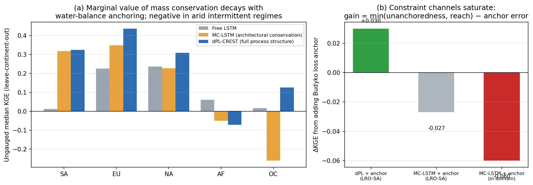
| Leave-out | Free LSTM | MC-LSTM | dPL | conservation buys |
|---|---|---|---|---|
| South America | 0.01 | 0.30 / 0.34 (2 seeds) | 0.32 | ≈100% of the gap |
| Europe | 0.23 | 0.35 | 0.44 | ≈half |
| North America | 0.21-0.24 | 0.23 | 0.31 | ≈zero - all structure |
| Africa | +0.06 | -0.05 (β0.57) | -0.07 (β0.39) | negative (under-delivery) |
| Oceania | +0.02 | -0.26 (β1.64) | +0.13 | negative (over-delivery) |
Three closed verdicts. (1) The in-distribution cost of architectural conservation (-0.11) is capacity-independent (32/64/128 cells: 0.42/0.42/0.42) - an intrinsic tax, not a size problem. (2) Conservation's marginal value decays monotonically with how water-anchored the target region already is, and turns negative in arid intermittent regimes - in both directions of failure. (3) Stacking a Budyko loss anchor on top of the conserving architecture adds nothing abroad (0.29 vs 0.30/0.34) and hurts at home (-0.06): constraint gain = min(channel unanchoredness, reach) - anchor error.