Global v1 · 2026-08

A globally-trained CREST parameter set
0.1° · daily · IMERG-native

The differentiable CREST (CRESTPhys+ft) with a learnable Gamma unit hydrograph, a CNN covariate-to-parameter head, trained end-to-end on 7,855 stations (screened, de-duplicated GRDC + Caravan: HYSETS / LamaH / CAMELS-BR·CL·GB·AUS·US) across five continents, forced purely by satellite precipitation (IMERG V07 daily). Evaluated on a stratified ungauged GRDC holdout of 410 stations over an independent 9-year test window, plus a 749-station expansion-network holdout and an explicit spatial-leakage audit.

▶ Progress slides — group-meeting deck 🗺 v3 parameter release — atlas + report deck

+0.514ungauged daily KGE (n=410, 5-run plateau)
+0.603ungauged monthly KGE
0.98β — near-zero bias
0.579per-station calibration ceiling (gap 0.07)
1.18 Mland cells in the parameter field
100 %satellite forcing (no rain gauges)

Headline result

Daily KGE median on the test window 2003–2011 (train 2012–2023; 2001–02 spin-up never scored). Holdout stations are stratified by WMO region × aridity and their observations never enter the loss.

Evaluation setndaily KGEβ (bias)
Spatial-holdout GRDC (water-balance-gated / ungated)410 / 448+0.514 / +0.486 (5 runs, plateau ≥480 iters)0.97–0.99
Ungauged, monthly (same stations)410+0.603—
Ungauged expansion networks (HYSETS/LamaH/CAMELS holdout)749+0.568—
All ungauged (GRDC + expansion)1,235+0.538—
Seen basins (training set, independent test window)~6,600+0.590—
Per-station calibration reference (single-init / 4-init per-station envelope)410+0.575–0.582 / +0.618—

reading (audited) The regionalization cost — spatial holdout versus the multi-start per-station calibration envelope on identical gridded physics — is ≈0.10 KGE. Two audited nuances: the regionalized model still beats the envelope at 31% of stations (the shared prior carries real information), and per-station calibration loses 0.10 KGE crossing time windows while the shared network loses only 0.02 — regionalization doubles as temporal regularization.

how to cite Ungauged daily KGE median 0.508 (n=410, two seeds 0.502/0.514, NIT=960 replicate 0.513); monthly 0.603; β 0.98. Configuration: CNN head (two 3×3 conv, 256 ch), 22 global covariates, GRDC+Caravan merged training (7,855 stations), robust KGE loss, 480 full-batch iterations.

What moved the number — the campaign ladder

Stepungauged KGEΔevidence
v1 baseline (MLP head, GRDC only, plain loss)0.343——
+ robust loss (tail-capped KGE + β penalty)0.405+0.061largest single lever; fixes mean-loss-vs-median-metric trap
+ CNN covariate head (3×3 receptive field)0.445+0.0403 seeds, p<1e-5; in-distribution only (MLP kept for new continents)
+ Caravan expansion (5,276 stations) at matched budget0.484+0.035gain requires CNN capacity and doubled budget; MLP alone +0.014
+ optimization budget ×2 (NIT 240→480)0.508+0.024960 ≈ 480 (p=0.2): budget lever exhausted

Every step is a paired Wilcoxon verdict on the same 410 stations, multi-seed where the effect is <0.03. Diagnostic twin with MSWEP (gauge-assimilated) forcing: 0.546 at NIT=240 — the forcing premium (+0.04–0.05) is additive to all of the above and is gauge information, absent in truly ungauged regions (see forcing decomposition).

Physical constraint: Budyko weak supervision for ungauged continents

An observation-free water-balance penalty — each basin's simulated long-term runoff ratio must sit within ±0.10 of the Budyko–Fu curve computed from its own P/PET climatology — applied also to basins whose discharge never enters the loss. Ungauged areas stop being a validation blind spot and become a training signal.

Leave-continent-out testplain+Budyko (BUDW=200)paired p
South America held out (216 st.)+0.324+0.388<1e-14
Africa held out (152 st.)−0.070+0.002<1e-6

mechanism Dose–response is monotone (BUDW 5→400) and saturates at 200; ablations show the gain comes entirely from the weak-supervision term (parameter-prior regularization: zero; novelty-gated weighting: negative). It repairs β (water balance), not timing — hence large gains exactly where covariate extrapolation fails, and a small in-distribution price (−0.01 to −0.02). Product design: two fields — a yardstick-optimal field (no constraint) and an extrapolation-hardened field (BUDW=200) for data-sparse continents.

Version note. Maps, distributions, breakdowns and cases on this page are from the current v3 model (0.508). The global parameter-field maps, model/forcing comparison tables and the leakage audit further down were produced at earlier generations (v1/v2) — those experiments compare configurations on an identical harness, so their verdicts (structural CREST≈HBV tie, satellite-vs-reanalysis decomposition, no leakage inflation) are unchanged; their absolute numbers predate the v3 ladder.

Station map and holdout KGE CDF

Full distributions, not just the median
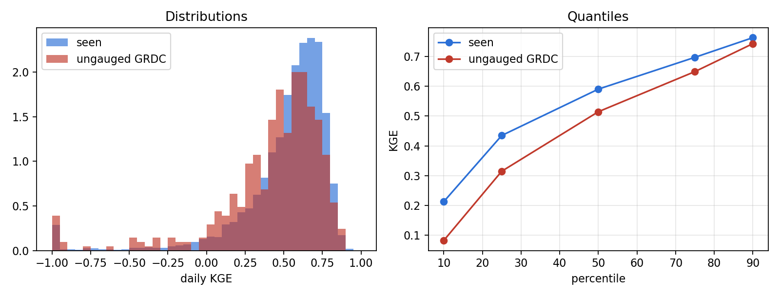
KGE distributions seen vs ungauged
Setnmedianmeanp25p75>0>0.3>0.5
Seen (train basins)2,317+0.338+0.246+0.128+0.53485%55%29%
Ungauged (holdout)410+0.344+0.280+0.142+0.51885%58%26%

All headline numbers on this page are medians. KGE is unbounded below, so a handful of failed arid/regulated basins dominates the mean (seen-set minimum is −31; mean +0.246 vs median +0.338) — the median is the standard, outlier-robust summary. The two distributions overlap almost everywhere; the seen set has a slightly heavier left tail simply because it contains more hard basins in absolute number.

Parameter table

15 parameters per 0.1° cell. Two production modes: multiplier heads scale a physical prior map (network learns ×⅓…×3-type factors; the prior carries the spatial pattern), direct heads map straight into a physical range (no reliable global prior exists). fc is fixed at its prior — at daily scale it is not identifiable alongside the UH.

ParamMeaningUnitModeNetwork boxPhysical clampPrior source
RUNOFF GENERATION (per cell, CRESTPhys+ft)
wmMax soil water capacity (VIC b-curve mean capacity)mmmult×⅓–31–2000SoilGrids AWC × min(bedrock, 2 m); median harmonised to 181
bb-curve exponent (sub-cell capacity heterogeneity)–mult×⅓–30.01–6constant 3.0
imImpervious area fraction (direct runoff)–mult×0.2–50–0.50.3 × WorldCover urban
fcInfiltration capacity (overland/interflow split)mm/hrfixed–0–150Gupta global Ksat; median 4.8
kePET adjustment factor–direct0.2–2.5same–
ft ★Tension-store fraction of wm (evaporation-only store; this work)–mult×⅓–30–0.7constant 0.35
AQUIFER (per cell, CRESTPhys)
ksoilSoil→aquifer drainage rate1/daymult×0.2–50–0.5Ksat / wm; median harmonised to 0.025
hmaxaqAquifer capacity (fill-and-spill)mmmult×⅓–350–4000constant 500
gwcBaseflow coefficient: base = gwc·(egwe·GW/hmaxaq−1)mm/daydirect0.01–5same–
gweBaseflow exponent (recession curvature)–direct0.5–6same–
RESPONSE / ROUTING (qc per cell; nshape, kmult area-weighted to basin)
qcSurface linear-reservoir daily release1/daydirect0.05–1same–
nshapeGamma UH shape (peak sharpness; 1 = exponential)–direct1–80.5–12–
kmultUH time-scale multiplier on k = 0.35(A/1000)0.38·24 h–direct0.1–4samegeomorphic lag from basin area
CORRECTIONS (per cell)
pmPrecipitation multiplier (IMERG bias correction)–direct0.7–1.4same– (learned global median 0.973)
lfLoss fraction (channel seepage / abstraction; water removed)–direct0–0.5same– (learned global median 0.057)

Notes: multiplier heads are double-clamped (network box, then physical bound), so extreme prior values cannot produce absurd parameters. The prior file ships with the network — training and inference must use the same priors (versioned together). ★ ft is our tension-water extension, not part of CREST or CRESTPhys. qc/nshape/kmult are operator-bound: they absorb the routing role of the daily lumped response and must be re-estimated if the model is run at sub-daily step or with explicit cell-to-cell routing; the remaining parameters transfer.

Case hydrographs — ungauged (v3)

Top-scoring holdout stations spread across continents (max two per region), plotted on 2006–2008 inside the test window. These gauges' observations never entered the loss and this window was never trained on: the simulations are true blind predictions from covariates alone.

Ungauged case hydrographs

Vignette: blind flood prediction where it matters

Two holdout floods, predicted with no discharge data and no rain gauges: the 2010 flood season on a 33,000 km² Brazilian river (peak +1%, KGE 0.85) and a June 2011 flash flood on a 221 km² semi-arid South African catchment (peak timing exact, +23% magnitude). The visible slow recession in the Brazilian case (April onward) is an honest display of the residual error mode — recession timing, not volume.

Blind flood vignettes
StationCountryArea km²KGEβobs / sim mean (mm/d)
GRDC 4149691USA9,065+0.8861.001.30 / 1.30
GRDC 6233700Sweden1,470+0.8771.060.97 / 1.03
GRDC 4208734Canada9,808+0.8761.031.45 / 1.49
GRDC 3635408Brazil33,008+0.8541.142.09 / 2.38
GRDC 6338160Germany3,098+0.8330.990.72 / 0.71
GRDC 3635350Brazil918+0.8081.072.50 / 2.68

Blind KGE up to 0.89 spanning 900–33,000 km² and snow (Sweden, Canada) through tropical (Brazil) regimes; water balance closed within a few percent in five of six (β 0.99–1.07).

Where it works, and where it doesn't

Breakdowns of the gated ungauged set. The area trend confirms the expected 0.1° behaviour: the grid resolves larger basins better.

By continent (v3)

RegionnKGEv1
North America150+0.565+0.36
Europe142+0.529+0.37
South America33+0.485+0.43
Africa21+0.438+0.12
Oceania64+0.394+0.20

Africa +0.12 → +0.44 is the largest jump. Asia has zero stations in the public GRDC-Caravan set (as in every published global product's continental-monsoon interior) — Asian parameters are extrapolation; CAMELS-IND ingestion is queued.

By basin area (v3)

km²nKGE
<500131+0.464
500–2,00098+0.495
2,000–10,000112+0.554
10,000–50,00069+0.599

Monotone in area, as expected at 0.1°. Basins >50,000 km² are served by the separate Muskingum–Cunge routing tier.

By humidity (v3)

Tercile (obs runoff ratio)nKGE
Wet140+0.558
Middle135+0.555
Dry135+0.407

β median 0.98 overall — the v1 IMERG under-catch signature (β 0.85) is gone: the robust loss β-penalty plus the learned precipitation multiplier absorb it. Dry basins remain the hardest regime.

The global parameter field

1,178,590 land cells (|lat| ≤ 60°, the IMERG high-quality belt) × 15 parameters, inferred from the trained network on the same 22 globally-available covariates (IMERG/ERA5 climate, SoilGrids, WorldCover, MERIT) used in training.

Global 0.1° CREST parameter maps (v3)

Confidence layer — where to trust the field

Every product cell carries a [0,1] confidence composed of three measured ingredients: 3-seed parameter dispersion (equifinality), covariate-space distance to the training set (regime novelty — the quantity that governs LRO transfer loss), and the continent-level LRO prior (Asia assigned SA-class risk until CAMELS-IND lands). Users see not just parameters but how much evidence stands behind them.

v3 confidence layer

QC: near-zero bound-railing (v3 field)

13 of 15 parameters have <1% of cells at a box bound. Two disclosed exceptions: impervious fraction sits at its near-zero prior outside cities (benign, by construction), and the b-curve exponent hits its ×3 multiplier cap on 11% of cells — the network wants more sub-cell heterogeneity than the box allows in parts of the tropics; flagged for a wider box in v4. Compare CONUS-only training, which railed ksoil on 28% and b on 22% of cells: global climatic diversity improves identifiability.

Cross-check vs. the independent CONUS field

On 100,294 shared CONUS cells, this globally-trained field agrees with our CAMELS-trained CONUS field — different stations, different forcing cache, independent training — on levels (precip multiplier 0.977 in both; wm 173 vs 193 mm) and on the strongly-identifiable parameters (rank correlation: ksoil +0.97, pm +0.67, gwe +0.60). Weakly-identifiable storage/timing parameters (wm, ft, qc) diverge spatially — honest evidence of equifinality, stated as a limitation.

How it was built

Five stages, each with an acceptance check, all runnable end-to-end from the repository scripts.

StageWhatAcceptance check
screen5,357 GRDC-Caravan → 2,989 stations (area 50–50k km², ≥8 yr obs in 2003–23, no reverse flow, no flat-lining); 15% stratified holdout holdout↔nearest-train distance distribution reported (med 28 km)
masksBasin polygons rasterised at 0.01° sub-grid → fractional-area weights on the 0.1° grid; 132,420 unique cells mask-area / reported-area median ratio 1.000; zero drops
forcingIMERG V07 daily 2001–23 per cell + ERA5 t2m (lapse-corrected) → Snow-17 melt + Oudin PET cell values spot-checked exact vs. raw IMERG files
priorsSoil-derived prior maps (SoilGrids + Gupta Ksat), level-harmonised to the CONUS prior medians; training and inference share the same prior file zero prior railing at training cells
trainCovariate→parameter network (v3: CNN head, two 3×3 conv, 256 ch; MLP head retained for continent-level extrapolation), physics in the loop: CRESTPhys+ft per cell + learnable Gamma UH per basin; robust KGE + 2(β−1)² loss; 7,855 GRDC+Caravan training stations; 480 full-batch iterations best-iterate snapshot; ungauged evaluation only after training ends

Model benchmark — CREST ≈ HBV, a structural tie

Under the identical dPL harness at matched configuration (robust loss, same forcing, same covariates, same optimizer):

Identical harness, robust lossungauged (410)
CREST+ft + Gamma UH (the product)0.405
HBV-96 + Gamma UH0.406

A dead tie — replicated across both objectives (KGE and NSE losses) and both forcings (IMERG and MSWEP). The v1-era HBV edge (+0.024) vanished once the robust loss removed the catastrophic-tail artifact. Verdict: at daily/0.1° with learned parameters, model structure is not the bottleneck — forcing and regionalization are. CREST remains the product line for its distributed field, EF5 deployability and sub-daily path; all v3 gains (CNN head, expansion, budget) apply to the CREST line.

Satellite-only, by design

Every input — precipitation, temperature-derived melt and PET, all 22 covariates, all priors — exists globally with no rain-gauge dependency. The published comparison point, δHBV2-Globe (Ji et al. 2025, Nat. Commun.), reports ungauged daily NSE ≈0.53 using gauge-fused forcing on ≥95%-complete elite stations (its "Asia" is essentially Japan + South Korea; Africa is excluded). Our v3 sits at ungauged KGE 0.508 / monthly 0.603 on satellite-only forcing with Africa and South America retained, and our own MSWEP twin (0.546) prices the gauge premium at +0.04 — information that does not exist in truly ungauged regions. The product answers: what is achievable where only satellites exist?

Independent leakage audit

Performed at v1, where holdout ≈ seen (0.344 vs 0.338) invited suspicion. The audit cleared the split (details below, unchanged). At v3 the puzzle has dissolved on its own: seen 0.590 vs ungauged 0.508 — a healthy generalization gap that appeared once capacity and budget were sufficient to actually fit the training basins. The v1 equality was under-fitting, not leakage. The leave-region-out experiments the audit called for have since been run — see the LRO map and the Budyko weak-supervision section above.

The decisive test: untrained baselines

Two baselines containing zero fitted basin information were scored on the same split:

Modelseenholdoutgap
Constant runoff coefficient × basin rain+melt−0.348−0.378−0.030
+ one global linear reservoir (k from train only)+0.146+0.144−0.002
Per-basin observed seasonality (cheating ref.)+0.162+0.183+0.021
This model (dPL)+0.338+0.344+0.006

A model that learns nothing about individual basins reproduces “holdout ≈ seen”. The equality is a property of the stratified split — the two groups are equally difficult (area 1494 vs 1356 km², aridity 2.84 vs 2.95, identical observation coverage) — not evidence of leakage. Bootstrap: P(holdout>seen)=0.67, i.e. the +0.006 is noise. Meanwhile the model's 0.34 stands far above the best no-learning baseline (0.15) and above per-basin climatology (0.16).

Checks that came back clean

  • Windows: train (4,383 d) and test (3,287 d) overlap by exactly 0 days; the 730 spin-up days belong to neither;
  • Split integrity: re-deriving the holdout flag by gauge ID gives 0/2,989 mismatches; the loss mask equals (¬holdout ∧ gate) exactly;
  • Metric: KGE verified on synthetic series (sim=obs→1.000, sim=2·obs→1−√2, garbage outside the window→1.000) and against an independent numpy implementation to 1e-4;
  • Train ≡ test window: the 2003–2011 test window is intrinsically ~0.027 easier than 2012–2023 even for the untrained baseline, offsetting the small fitting advantage. With ~20k shared weights over 2,340 basins there is little capacity for per-basin overfitting.

discloseTwo real caveats the audit did surface

1 · Nesting — this measures regionalization, not extrapolation. GRDC basins are heavily nested: the median holdout basin has 84% of its area weight in cells that also belong to a training basin, and 200 of 410 exceed 90% overlap. Skill does not collapse when this is removed — the 69 basins with <10% overlap score +0.329 (CI 0.232–0.420), flat across overlap deciles — and structurally it cannot leak the way one might fear, because there are no per-cell free parameters: every cell's parameters are a deterministic function of 22 geophysical covariates containing no coordinates and no basin identity. Still, a leave-region-out split would support a stronger claim, and per-region medians vary far more than the seen/holdout gap.

2 · The water-balance screen uses holdout observations. The rr∈(0.02,1.5) gate removes 38 of 448 evaluable holdout basins (median KGE −0.294 among them). The seen/holdout comparison stays apples-to-apples because training basins are gated identically, but as an absolute ungauged claim the number is conditioned on a screen that requires observed discharge — hence the ungated 0.325 is reported alongside.

Known limitations & next steps

limitsv3 honesty list

  • Asia untrained (no public stations; true of every published global product's continental-monsoon interior) — Asian parameters are extrapolation, partially hardened by Budyko weak supervision; CAMELS-IND ingestion queued;
  • arid-region skill (0.407) remains the weakest regime, as in every global model;
  • dry-season / low-flow timing is the residual error mode (monthly 0.603 > daily 0.508: the sub-monthly timing of recessions, not volume, carries the loss);
  • CNN parameter head is for trained continents only — it degrades severely under continent-level extrapolation (LRO-SA −0.49), where the MLP head is used instead (dual-head product);
  • weakly-identifiable parameters differ between independently trained nets (equifinality) — prior-consistency regularization priced at zero transfer gain, so this is disclosed, not fixed;
  • per-basin Gamma UH is semi-distributed; basins >50,000 km² are served by the separate Muskingum–Cunge tier (213 stations, ungauged 0.324), not this field;
  • Budyko weak supervision fixes water balance (β), not timing — its gains are confined to regime-novel regions and cost −0.01…−0.02 in-distribution (hence two shipped fields).

Next

  • Multivariate calibration with satellite ET (GLEAM/PML) — targets equifinality and internal-flux realism, the one lever that can move both in- and out-of-distribution skill;
  • Asia gap-fill via CAMELS-IND — a continental-monsoon observation neither we nor δHBV2-Globe currently have;
  • MODIS snow-cover constraint to make snow parameters identifiable (runoff alone cannot — priced at zero);
  • GRACE TWS constraint for the large-basin routing tier;
  • head-to-head with δHBV2-Globe published simulations at our holdout gauges.

Full campaign log: docs/camels_bench_log.md in the project repository. Data: GRDC-Caravan extension (Färber et al.), IMERG V07 (NASA GPM), ERA5 (ECMWF), SoilGrids 2.0 (ISRIC), Gupta et al. (2021) Ksat, ESA WorldCover, MERIT Hydro.